Abe N., Tsukahara M., Homma F., Omomo Y., Ishiyama T. The System for Assessment of the Japanese Cedar Forest Resources Using Space Image Data

Article

---

INTRODUCTION

Japanese cedar (Cryptomeria japonica (Thunb. Ex. L. f.) D. Don), “sugi” in Japanese) is the most economically important plantation tree in Japan. The area of sugi plantations is approximately 40 % of the whole manmade forest area in Japan (Forestry Agency, 2012) (Fig. 1). 

 

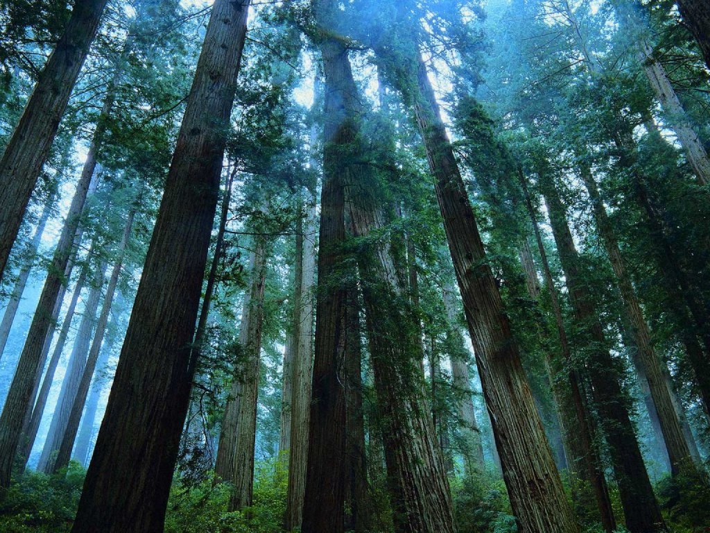
Fig. 1. Planted, 70 year old sugi forest in Niigata prefecture.
 

Many sugi stands have matured to cutting age, but the timber price is sluggish and we need to reduce cutting expenses to promote their practical use. In Japan, the forest basic map and forest register are used for management of manmade forests. However, volume in the register is calculated using the growth curve incorporated into the database, and differs from the actual volume. There are some reports that estimate the volume of sugi plantation using space image data (Abe, Ishida, 2004; Abe, Iida, 2009). The Landsat space image has been used to estimate the forest volume in the past. However, the Japanese satellite ALOS (Advanced Land Observing Satellite) has not been used for this purpose. The accuracy of the estimate may vary with the satellite. In this study we used ALOS to estimate the volume of sugi forest.

The objectives of this research are:

a) to evaluate the best-fit equation model for the timber volume between digital number and volume per hectare;

b) to investigate factor on the accuracy for equation, and

c) to increase the accuracy of forest register using satellite information.

  

MATERIALS AND METHODS

The study area is located in Jhoetsu district, Niigata Prefecture, and covers approximately 2165 km². Image data sets used in this study were obtained from ALOS satellite by AVNIR-2 (Advanced Visible and Near Infrared Radiometer), and  PRISM (Panchromatic Remote Sensing Instrument for Stereo Mapping). PRISM was used to construct pan-sharpened images. The acquisition metadata of ALOS satellite are shown in Table 1.

 

Table. 1. ALOS acquisition metadata 

Characteristics	AVNIR-2	PRISM
Observation Date	2010/5/8	2010/5/8
Center Longitude	138.1020	37.2095
Center Latitude	37.2439	37.2095
Resolution	10 m	2.5 m
Area covered	70 km	70 km
Band	BAND1, 0.42～0.5μm BAND2, 0.52～0.6 BAND3.0.61～0.69 BAND4, 0.76～0.89	BAND1, 0.5～0.77μm

 

  

 

The vegetation in the study area consists of coniferous and broadleaved species. Coniferous species are sugi (Cryptomeria japonica (Thunb. Ex. L. f.) D. Don)), akamatsu (Pinus densiflora Siebold et Zucc.), kuromatsu (Pinus thunbergii), Norway spruce (Picea abies (L.) Karst.)), etc. Broadleaved species are buna (Fagus crenata Blume), mizunara (Quercus mongolica Fisch. ex Ledeb.), hounoki (Magnolia obovata), tochinoki (Aesculus turbinata Blume), etc. (MSCIE, 1995).

For image processing we used ERDAS ver. 9.1 (ESRI, 2009), for topographic processing the digital map, and for geometric correction, the 1/5000 scale forest basic map. The basic map was transferred to GIS. For topographic correction, the digital map (50 m mesh, Geospatial Information, 2009) was used. Plots were established based on the Niigata Prefecture Forestry Division method (plot size was 40 m × 40 m, tree height and stem diameters were measured for each tree).

1) Removal of small pixels method

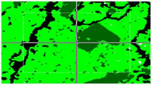
This paper deals to extract forest by supervised classification. Classification of image usually is made on pixel units, but it includes differently classified small pixels. Therefore, to classify the area smoothly, we used ERDAS (ESRI, 2009) which has a function to classify the pixel image smoothly. This function uses digital numbers of circumferential 25 pixels focusing on a certain pixel, and modify the classification using the most frequent pixel value. Thus, we can make thematic images smoothly to delete the small classified pixels. Usual classification figures before and after removal of small pixels are shown in Figure 2. Figure 2 b looks much close to natural condition.

 

                                            a                                                                                     b

      
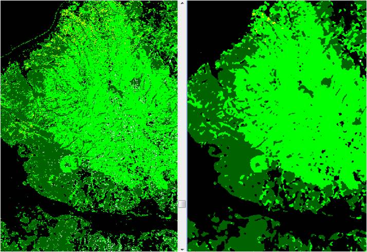
Fig. 2. The procedure for removal of small pixels: a – usual classification; b – classification by removal of small pixels.

 

2) RPC (Rational Polynomial Coefficients) geometric correction

We used the ALOS image after RPC geometric correction (RPC file). This RPC file is made from the projection model using an approximate polynomial curve coefficient. Approximation by RPC data is shown by rational function of standardized latitude, longitude and altitude, and is given by the standardized polynomial coefficient (EORC/RESTEC 2009).

Usually, the accuracy of geometric correction is shown by RMSE (Root-Mean-Square Error), but not by RMSE when RPC is used. RMSE value is desirable within 0.5. But, this time, RMSE value was 13.2532 in AVNIR-2 and 17.5745 in PRISM by ERDAS (2009). This cause have not been discovered.

4) Application of pan-sharpen image

Monitoring by visual image is also important, since resolution of AVNIR-2 of ALOS (10 m × 10 m) is not high enough. However, pan-sharpen image made by using AVNIR-2 and PRISM has adequate resolution (2.5 m × 2.5 m) (Fig. 3).

                а)                                                                                   b)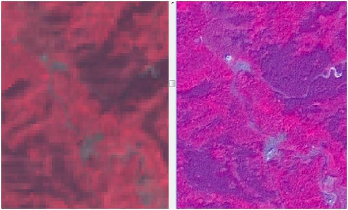

Fig. 3. AVNIR-2 (a) and PRISM pan-sharpened (b) scenes.

 

Thus, we can visually decipher forest, road, sugi stand, and broadleaved stand. Pan-sharpen image is precisely corrected geometrically by AVNIR-2 and PRISM, and the pan-sharpened image is useful to take training area polygons in the scene. 

 

RESULTS

1) Geometric correction

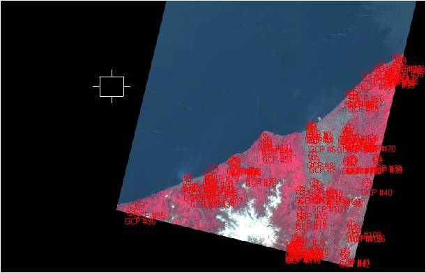
It was inadequate to show accuracy of geometric correction using RMSE in case of RPC file. This is because the RPC model shows good correlation between the image and map for flat ground but not mountainous areas. In this study, the majority of the study area is mountainous. Therefore, geometric correction was performed by using more than 60 ground control points (GCP) for AVNIR-2 and PRISM images. We checked various points image and map using geo-link (Fig. 4).

 

                                                                   AVNIR-2                                                     

 

                                                                      PRISM

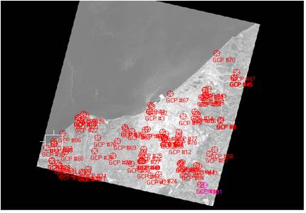
Fig. 4. Location of GCP at AVNIR-2 and PRISM scenes.

    

Here, the geo-link image in the mountainous area is shown (Fig. 5). Other point showed same accuracy.

 

                                       AVNIR-2                                                     Topographic map of 1 : 5000 scale

  

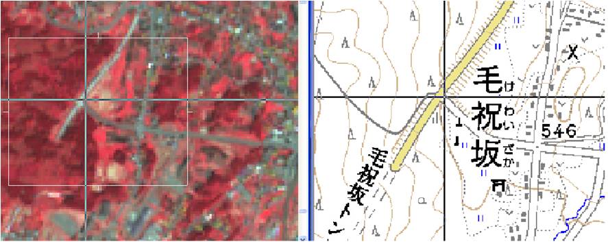
Fig. 5. AVNIR-2 scene after geo-link and map GCP positioning correction. Sign “十” shows same points’ coordinates on image and on the map.

  

2) Topographic correction

In mountainous areas, topographic correction is indispensable. The correlation coefficient between sugi forest volume corrected by various topographic correction methods and wavelength of band used has been reported by R. Riva and N. Abe (2006). Topographic correction methods used were Static Empirical method, Minnaert Correction method, C-Correlation method and Topographic Normalize method. Coefficient of correlation of volume with digital number of various bands (band value) was highest with band 1 by Topographic Normalize method, band 2 by Topographic Normalize method, band 3 by C-Correction method, band 4 by C-Correction method, band 5 by Minnaert correction method, and band 7 by the Minnaert Correction method. However, since the difference in the correlation coefficient was slight, the most common method Minnaert Correction method was used in this study. In this method, however, topographic correction is impossible in the area without direct incident rays, i.e., cosine (cos) of incidence angle is negative. To cover this defect, we used the Dual Partitioning Regression method (Sakamoto et al., 2009) separating the area into two areas: cosi > 0 and cosi < 0. After topographic correction, we obtained a larger digital number than before correction. The parameters of Dual Partitioning Regression with (obtained by using) the digital number of bands 1 (9.3864), 2 (28.9788), 3 (28.251) and 4 (54.1233). Figure 6 shows ALOS image after topographic correction by Dual Partitioning Regression and Minnaert.

                                           a                                                                                      b

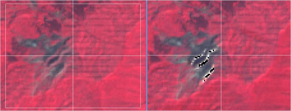
Fig. 6. Topographic correction of ALOS scene by the Dual Partitioning Regression method (a), and by Minnaert method (b).

  

3) Supervised Classification

This study aims at estimating the sugi stand volume. Therefore, forests were extracted by primary classification, and then sugi stands from the forest by secondary classification. Supervised classification has two methods. One is parametric method and the other is non-parametric method. In this study, we used Maximum Likelihood Classification and Mahalanobis Distance Method as parametric method, and multilevel slice classifier method as non-parametric method. We calculated overall accuracy of the three methods. As a result, in primary classification the Maximum Likelihood Classifier showed the highest (94 %) classification accuracy, and k (Lillesand and Kiefer, 2000) = 0.867. In secondary classifications, the Mahalanobis distance method showed 89 % accuracy for forest but 68 % accuracy for sugi stand and k (“KHAT”statistic, Lillesand and Kiefer, 2000) = 0.6085. So, we adopted the Maximum Likelihood Classifier as primary classification and Mahalanobis Distance Method as secondary classification.

The scenes of primary and secondary classification areas are shown in Figures 7 and 8, respectively, and the area of land categories and forest types in ha by spectral class of primary and secondary classifications are shown in Tables 2 and 3, respectively. In both tables, the forest area was 110 975 hectare.

 

 

Fig. 7. Primary classification of the land categories.
 
    

  

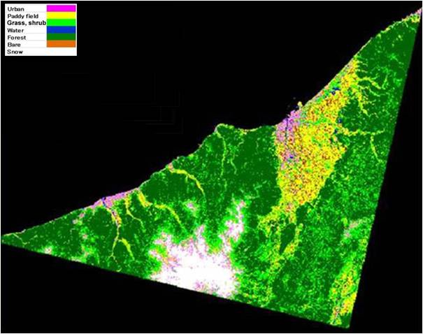
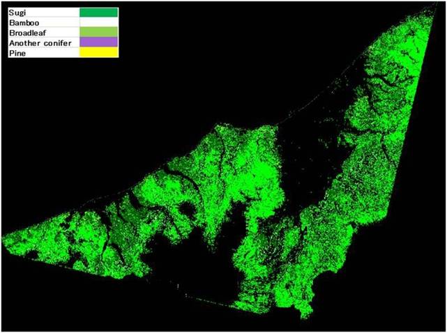
Fig. 8. Secondary classification of forest types.

  

Table. 2. The area of land categories by spectral class of primary classification

 

Table. 3. The area of tree stands by spectral class of secondary classification

Types of a tree stands	Area, ha (%)
Sugi (Crytomeria japonica D.Don)	35 991 (32.4)
Broadleaf	69 366 (62.5)
Pine (Pinus Thunbergii and P. densiflora)	498 (0.45)
Another conifer (Picea abies)	1 581 (1.42)
Bamboo (Bambusa metake)	3 539 (3.23)
Total	110 975 (100)

 

   

 

4) Construction of equation to estimate sugi stand volume

To analyze regression equation between digital number of space image data and volume, we used the past plot data of sugi monitoring, plot data of old-aged sugi forest, inspection plot data of volume for register, and this year plot data of sugi monitoring. Total plots were 58 plots. It was necessary to obtain average digital number for each plot. Thus, we used ERDAS (ESRI, 2009) which has a region growing tool to average the digital number in the fixed range. The fixable number needs to be fixed to use this region growing tool. The average digital numbers using 100 pixels was similar to that using 20 pixels (Fig. 9).

 

                                          a                                                                                    b

 

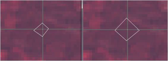
Fig. 9. The aggregate by spectral class areas on ALOS scene, allocated by region growing tool for 20 pixels (a), and 100 pixels (b).

  

Therefore, I used 20 pixels considering plot area (100 m × 100 m ~ 50 m × 50 m), and resolving power of ALOS (10 m × 10 m).

Parameters effective for estimating volume per plot were selected by multiple regression analysis between volume per plot and average digital number per plot. All plots were used for regression analysis, and the effective band was selected by the stepwise procedure (SPSS, 2009). The significantly effective band for volume estimation was band 4 as shown in Table 4.

  

Table. 4. The parameters for estimating volume (V) per plot selected by multiple regression and stepwise procedure

Equation	Sum of squares	Degrees of freedom	Average sum of squares	Fischer coefficient	Significance Pro.
V = 1010.823 – 7.297 Band 4
Regression Residual Total	280668.51 4421442.4 4702110.91	1 57 58	280668.51 77569.16	3.618	0.062
V = 945.494 – 7.521 Band 4 + 1.239 Band 3
Regression Residual Total	282280.16 4419830.7 4702110.86	2 56 58	141140.079 78925.549	1.788	0.177
V = 1180.662 – 7.659 Band 4 + 2.529 Band 3 – 2.702 Band 1
Regression Residual Total	286535.417 4415575.46 4702110.88	3 55 58	95511.806 80283.19	1.19	0.322
V = 1671.485 – 15.130 Band 4 – 11.503 Band 3 – 24.003 Band 1 + 37.970 Band 2
Regression Residual Total	326182.000 4375928.88 4702110.88	4 54 58	81545.5 81035.720	1.006	0.412

 

 

Analysis of variance shows that the regression equation is significant, but coefficient of correlation was not high. In this case, the multiple correlation coefficient was 0.2595 (Table 5).

 

Table. 5. Analysis of variance of the regression equation

Equation V = 1010.823 – 7.297 Band 4	SS	DF	Mean square	F	Significance Pro.
Regression Residual Total	434550.655 4267560.227 4702110.881	1 57 58	434550.655 74869.478	5.804	0.019*

* 1 / Band 4

    

On the other hand, NDVI (Nomalized Difference Vegetation Index）is known as an effective index for analyzing vegetation. When volume is shown as a function of bands 1, 2, 3 and 4 and NDVI, and analyzed by a stepwise procedure, the significant variable (at 5 % level) was only Band 4 (F value 3.618). The highest correlation coefficient (r = 0.304) was obtained by the following formula and showed analysis of variance on Table 5.

Figure 10 shows the correlation between volume and reciprocal of band 4 value, and Table 6 shows the area with estimated volume classes obtained using above equation.

  

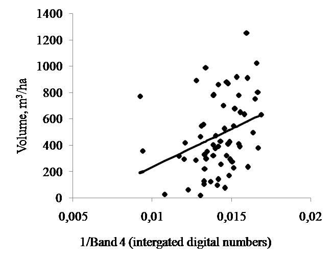
Fig. 10. Relationship between sugi tree stand volume and reciprocal of band 4.

  

Table. 6. Estimated sugi tree stand volume class and the area

Volume class, m3/ha	Area, ha (%)
Under 200	0.21 (0)
201～300	187.6 (0.5)
301～400	10 149 (28.2)
401～500	8 041 (22.3)
501～600	7 843 (21.8)
601～700	6 598 (18.3)
701～800	2 762 (7.7)
Over 800	410.19 (1.2)
Total	35 991 (100)

 

 

As shown in Figure 11, estimated sub-compartment volume was sometimes close to actual sub-compartment value but sometimes excessive or underestimate.

 

                                                                                   AVNIR-2

                                                                        Secondary classification 

                                                                  The volume distribution map

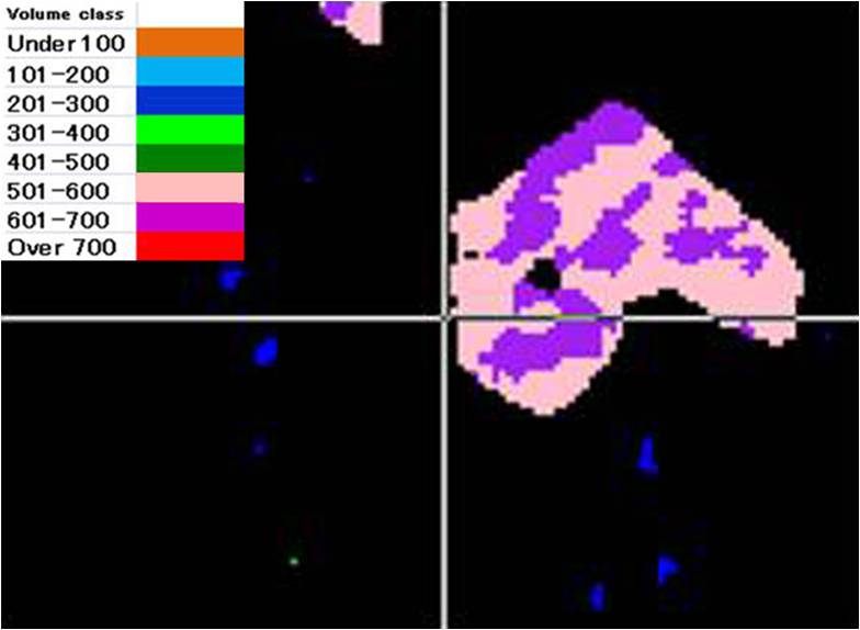
Fig. 11. Plot number 7, sugi tree stand volume is 389.5 m³/ha, as shown in the forest register.

  

In forest register, sub-compartment is shown as the spot with the same volume, but from satellite data various volumes were estimated in the same sub compartment. Considering the geographical feature of each sub-compartment, it is more natural that the volume is variable in the same sub-compartment, because growth is uneven in a small spot.

5) Criterion of non-vegetation by NDVI

Table 7 shows the areas with different NDVI classes in the sugi forest register.

 

Table 7. Areas of NDVI classification of sugi forest

  

NDVI class	Area, ha
Under 0.053	604.09
-0.052~0	3198.7
0.0001～0.00856	1096.5
0.00087～0.0444	5287.9
0.0445～0.0856	6176.9
0.0857～0.1344	6611.1
0.1345～0.1941	7663.7
Over 0.1942	2664.6

 

 

   

 

Using these NDVI classes, we can show the distribution of different NDVI classes in the forest (Fig. 12). The left half of the figure shows sugi stand information by register, and right half NDVI diagram. Red color means positive NDVI, which is vegetation area, and the false color shows negative NDVI, which is the non-vegetation area. Thus, we can check non-vegetation area easily as shown in Figure 12. The negative value of NDVI shows a non-vegetation area such as forest road and timber yard.

 

                                     False color                                                                  NDVI class

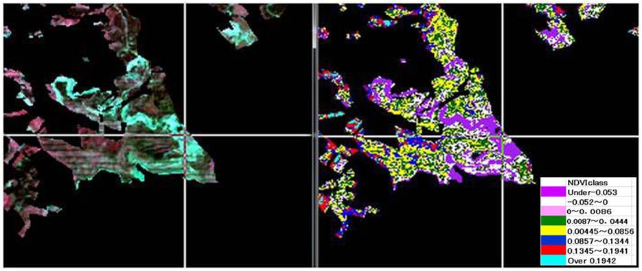
Fig. 12. NDVI classification of sugi forest.

  

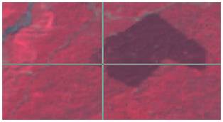
We have examined AVNIR-2 space image data, where we can see light blue areas by false color. Light blue color means areas not covered by sugi forest, but they are applicable to forest road, timber yards, glades etc. And we showed digital number of that areas. ALOS band 1 is blue, band 2 – green, band 3 – red, and band 4 – near infra red. Band 1 value is 150, band 2 –142, band 3 –143, and band 4 – 71. So, NDVI value is –0.3364. Figure 13 shows digital number of each band of pixel.

  

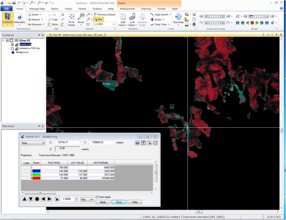
Fig. 13. Comparison of ALOS (AVNIR-2 digital numbers.

  

DISCUSSION

In our previous study with space images, the study area was often small watershed (Abe and Ishida, 2004, Riva and Abe, 2006). In this study, therefore, we attempted to estimate the sugi stand volume in the ALOS full scene range.

In many previous studies, the Landsat satellite was used to estimate forest volume and studies were focused on the effective band (bands 1, 2, 3, 4 ….).

C. B. Puhr and D. N. M. Donoghue (2000) reported the relationship between estimated basal area and each band value using the Landsat TM data. Significant correlation was observed with bands 3, 5 and 7 values but not with band 4 value.

J. Franklin (1986) and J. Ardö (1992) have also reported that the correlation between volume and band 4 value is low.

C. B. Puhr and D. N. M. Donoghue (2000) explained that the reason for the low correlation coefficient is that the influence of diffused light of SWIR is smaller than that of TM band 4 values. However, there are many reports showing that the correlation coefficient of volume with TM band 4 value is higher than that with other band values.

C. M. Trotter et al. (1997) reported that only bands 3 and 4 were selected as effective by the step-wise method, but the coefficient of determination was 0.3. F. J. Ahern et al., (1991) reported that the correlation coefficient between net annual volume change and band 4 reflectance was > 0.8 in spruce-fir stand. In addition, they reported that live spruce-fir volume was closely correlated with band 4 reflectance.

M. A. Spanner et al. (1990) reported that the volume of stand with low Leaf area index (LAI) was closely correlated with the values of bands 3 and 5, but that of the stand with high LAI with band 4 values.

In the report of R. Riva and N. Abe (2006), the correlation coefficient of volume with the values of bands 4 and 5 was nearly the same, 0.735 and 0.766, respectively.

J. Ardo (1992) reported that the correlation coefficient between volume and band value is higher in a small volume stand than in a large volume stand.

F. Gemmel  (1995) reported that the correlation was lower in the stand with over 400 m³ volume stand.

It is considered that the correlation between band value and volume is greatly influenced by the forest conditions. Various forests were used in this study from boreal forest (Ahern et al.,1991) to radiata pine (Pinus radiata D. Don)  (Trotter et al., 1997). It is considered that the accuracy of the estimation of volume by using band values varies with the tree species, understory vegetation, forest type and the volume class. Thus, it is necessary to accumulate these data in the future.

In this study using ALOS, correlation coefficient between volume and band 4 value was low though statistically significant. This may be because the study area was wide including various sugi stands.

Table 8 shows the coefficient of variation range of volume estimated using each band.

 

Table 8. Coefficient of variation range of each band and volume

Band 1	Band 2	Band 3	Band 4	Volume, m3/ha
3.24%	4.61%	6.74%	15.83%	59.66%

  

 

The coefficient of variation of the volume estimated using each band was 3.24 – 15.83 %, but that of volume per hectare was as large as 59.66 %.

Thus, the variability of volume estimated using each band was smaller than that of volume per hectare. This difference is considered to reduce the correlation coefficient between volume and band 4 value. The variation of volume per hectare is biological variation, but the variation of band value (digital number) is physical. The reason for the low correlation coefficient between volume and band 4 value may be that the large variation of volume per hectare was not expressed by band 4 value due to its small variation. Why variation of band 4 value (digital number) was smaller than that of volume must be clarified in the future. C. B. Puhr and D. N. M. Donoghue (2000) reported that the variation range of the band value of SWIR was larger than that of forest structure.

Abe et al. (2004 and 2009) examined what bands are effective in estimating volume using a high-resolution satellite, and showed that only the band 3 value showed significant correlation with volume, which is different from the result of this study using ALOS. The resolution of ALOS is 10 m, which is intermediate that between the resolution of the Landsat and high resolution satellite Quiсk Bird. The relationship between volume and band value may be affected by resolution of the satellite in addition to band, forest type, tree species, understory vegetation and others. It is necessary to verify the results by increasing the number of analyses.

Japan has a forest resource database system, but it is not easy to check the contents of the register. The construction of a system that can point out the mistake of the register using a space image is very important. As shown in this study, the area where the NDVI value is negative is not a sugi forest. The negative NDVI value means that the band 3 value is larger than the band 4 value. It is well-known that the band 4 value is large in a vegetation area. Thus, the area with a negative NDVI is a forest road, timber yard, felling area, etc., which need to be corrected in the register. This means that the register can be corrected by using periodical satellite information and this greatly contributes to encouraging the practical use of sugi forests.

  

CONCLUSION

In the present study, the volume of sugi forests distributed in a wide area including mountainous area was investigated using the space image. The relationship between volume and reciprocal of band 4 value (digital number) was significant, but the correlation coefficient was low (r = 0.3). The coefficient of variation of volume was larger than that of the digital number of each band (band value). The low correlation coefficient between volume and band value may be attributed to smaller variation range of digital number compared with that of volume. On the other hand NDVI is an effective index of vegetation area. We showed that the area with a negative NDVI value is not a sugi forest. Improvement of the accuracy of sugi forest data base by using these methods may contribute to encouraging practical use of a sugi forest.

  

ACKNOWLEDGEMENTS

We used sugi stand data collected by Niigata Prefecture employees. We would like to thank the erosion control staff of Niigata Prefecture.

  

LITERATURE CITED

Abe N., Iida K. Estimation of carbon stock in even-aged sugi forests using satellite image data // J. Integr. Field Sci. 2009. V. 16. P. 9–13.

Abe N., Ishida T. Estimation of carbon stock in sugi plantations using high-resolution Quick Bird images // The role of forests for coming generations: philosophy and technology for forest resource management: Proc. int. symp. / Ed. by Kenji Naito. Tokyo, Japan: Jap. Soc. For. Plann. Press Publ., 2004. P. 221–229.

Ahern F. J., Erdle T., Maclean D. A., Kneppeck I. D. A quantitative relationship between forest growth rates and Thematic Mapper reflectance measurements // Int. J. Rem. Sens. 1991.V. 12. P. 387–400.

Ardo J. Volume quantification of coniferous forest compartments using spectral radiance recorded by Landsat Thematic Mapper // Int. J. Rem. Sens. 1992. V. 13. P. 1779–1786.

EORC/RESTEC PRISM/AVNIR-2 Level 1B2 RPC Data set // Report about making RPC data and inspection accuracy of RPC. 2009. 1–21 p.

ESRI Japan Inc. // ERDAS IMAGINE Manual 9.1.2009．

Forestry agency annual report on forest and forestry in Japan // Fiscal Year 2012. http://www.rinya.maff.go.jp

Franklin J. Thematic Mapper analysis of coniferous forest structure and composition // Int. J. Rem. Sens. 1986. V. 7. P. 1287–1301.

Gemmel F. Effects of forest cover, terrain, and scale on timber volume estimation with Thematic Mapper data in a Rocky Mountain site // Rem. Sens. Environ. 1995. V. 51. P. 291–305.

Geospatial Information Authority of Japan. Digital Map. 2009.

Lillesand T. M., Kiefer R. W. Remote Sensing and Image Interpretation. 4th Edition. New York; Chichester: Wiley, 2000. 724 p.

MSCIE (Meeting of Sugi Characteristics Investigation and Examination) // Sugi of Niigata Prefecture. Niigata Forestry Association for Improvement of Niigata Prefecture. 1995. Niigata (in Japanese).

Puhr C. B., Donoghue D. N. M. Remote sensing of upland conifer plantations using Landsat TM data: a case study from Galloway, south-west Scotland // Int. J. Rem. Sens. 2000. V. 21: 633–646.

Riva R., Abe N. Topographic correction effect on sugi (Cryptomeria japonica D. Don.) stand volume estimation using multi temporal Landsat TM and ASTER satellite images in mountainous Tsugawa Region, Niigata Prefecture // J. For. Plan. 2006. V. 12. P. 49–58.

Sakamoto K., Nakayama D., Matsuyama H. New topographic correction method of satellite image in the season of low solar elevation // J. Rem. Sens. Soc. Jap. 2009. V. 29. P. 472–484 (in Japanese with summary in English).

Spanner M. A., Pierce L., Peterson D. L., Running S. W. Remote sensing of temperate coniferous forest leaf area index. The influence of canopy closure, understory vegetation and background reflectance // Int. J. Rem. Sens. 1990. V. 11. P. 95–111.

SPSS 15.0J for Windows, 2009.

Trotter C. M., Dymond J. R., Goulding C. J. Estimation of timber volume in a coniferous plantation forest using Landsat TM // Int. J. Rem. Sens. 1997. V. 18. P. 2209–2223.